understand axis in matplotlib

axis is a subarea within figure() in matplotlib

figure()

plt.axes([0.3, 0.5, 0.4, 0.2])
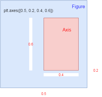


the figure area size is 1, 1 as base


In [2]:
import matplotlib.pyplot as plt
import numpy as np
In [6]:
physical_sciences=[ 13.8,  14.9,  14.8,  16.5,  18.2,  19.1,  20. ,  21.3,  22.5,
        23.7,  24.6,  25.7,  27.3,  27.6,  28. ,  27.5,  28.4,  30.4,
        29.7,  31.3,  31.6,  32.6,  32.6,  33.6,  34.8,  35.9,  37.3,
        38.3,  39.7,  40.2,  41. ,  42.2,  41.1,  41.7,  42.1,  41.6,
        40.8,  40.7,  40.7,  40.7,  40.2,  40.1];
computer_science=[ 13.6,  13.6,  14.9,  16.4,  18.9,  19.8,  23.9,  25.7,  28.1,
        30.2,  32.5,  34.8,  36.3,  37.1,  36.8,  35.7,  34.7,  32.4,
        30.8,  29.9,  29.4,  28.7,  28.2,  28.5,  28.5,  27.5,  27.1,
        26.8,  27. ,  28.1,  27.7,  27.6,  27. ,  25.1,  22.2,  20.6,
        18.6,  17.6,  17.8,  18.1,  17.6,  18.2]
year=[1970, 1971, 1972, 1973, 1974, 1975, 1976, 1977, 1978, 1979, 1980,
       1981, 1982, 1983, 1984, 1985, 1986, 1987, 1988, 1989, 1990, 1991,
       1992, 1993, 1994, 1995, 1996, 1997, 1998, 1999, 2000, 2001, 2002,
       2003, 2004, 2005, 2006, 2007, 2008, 2009, 2010, 2011]

two methods to specify many distinct graphs

In [10]:
# Plot in blue the % of degrees awarded to women in the Physical Sciences
plt.plot(year, physical_sciences, color='blue')

# Plot in red the % of degrees awarded to women in Computer Science
plt.plot(year, computer_science, color='red')

# Display the plot
plt.show()
In [8]:
# Create plot axes for the first line plot
plt.axes([0.05,0.05,0.425,0.9])

# Plot in blue the % of degrees awarded to women in the Physical Sciences
plt.plot(year,physical_sciences, color='blue')

# Create plot axes for the second line plot
plt.axes([.525,0.05,0.425,0.9])


# Plot in red the % of degrees awarded to women in Computer Science
plt.plot(year,computer_science, color='red')


# Display the plot
plt.show()
In [9]:
# Create a figure with 1x2 subplot and make the left subplot active
plt.subplot(1,2,1)

# Plot in blue the % of degrees awarded to women in the Physical Sciences
plt.plot(year, physical_sciences, color='blue')
plt.title('Physical Sciences')

# Make the right subplot active in the current 1x2 subplot grid
plt.subplot(1,2,2)


# Plot in red the % of degrees awarded to women in Computer Science
plt.plot(year, computer_science, color='red')
plt.title('Computer Science')

# Use plt.tight_layout() to improve the spacing between subplots
plt.tight_layout()
plt.show()
In [ ]:
 

more visualization

Time series

image wrangling

In [1]:
import pandas as pd
import matplotlib.pyplot as plt
% matplotlib inline
from yahoo_finance import Share
import numpy as np
In [2]:
btx=Share('BTX')
df=pd.DataFrame(btx.get_historical('2016-01-01','2016-04-01'))
df['Date']=pd.to_datetime(df['Date'])
df.dtypes
Out[2]:
Adj_Close            object
Close                object
Date         datetime64[ns]
High                 object
Low                  object
Open                 object
Symbol               object
Volume               object
dtype: object
In [3]:
df.index=df['Date']
df=df.drop(['Date','Symbol'],axis=1)
In [4]:
df.head(3)
Out[4]:
Adj_Close Close High Low Open Volume
Date
2016-04-01 2.92 2.92 3.02 2.84 2.90 281100
2016-03-31 2.87 2.87 2.90 2.76 2.83 277800
2016-03-30 2.77 2.77 2.83 2.65 2.70 239900
In [5]:
plt.plot(df.iloc[:,:-1])
plt.legend(['Adj_Close','Close','High','Low','Open'])
Out[5]:
<matplotlib.legend.Legend at 0x7f16d7c191d0>

Plotting an inset view

In [6]:
plt.plot(df['2016-01']['Open'])
plt.xticks(size=7, rotation=40)

plt.axes([0.55,0.4,0.3,0.45])
plt.plot(df['2016-02']['Open'],color='red')
plt.xticks(size=5, rotation=25)
Out[6]:
(array([ 735997.,  736000.,  736003.,  736006.,  736009.,  736012.,
         736015.,  736018.,  736021.]), <a list of 9 Text xticklabel objects>)

Time series with moving windows

numpy array.flatten()

Image histograms

Cumulative Distribution Function from an image histogram

  • A histogram of a continuous random variable is sometimes called a Probability Distribution Function (or PDF).
  • The area under a PDF (a definite integral) is called a Cumulative Distribution Function (or CDF). The CDF quantifies the probability of observing certain pixel intensities.
    • The histogram option cumulative=True permits viewing the CDF instead of the PDF.
In [7]:
orig = plt.imread('cat.jpg')
print orig.shape
pixels = orig.flatten()
print len(pixels), pixels.max(), pixels.min()
(194, 259, 3)
150738 255 0

plt.twinx()

  • The command plt.twinx() allows two plots to be overlayed sharing the x-axis but with different scales on the y-axis.
In [8]:
# Display a histogram of the pixels
plt.hist(pixels, bins=64, range=(0,256), normed=False,
 color='red', alpha=0.3)

# Use plt.twinx() to overlay the CDF 
plt.twinx()

# Display a cumulative histogram of the pixels

plt.hist(pixels, bins=64, range=(0,256), normed=True,cumulative=True,
 color='blue', alpha=0.3)
plt.title('PDF & CDF (original image)')

plt.show()

Equlize the image

  • Histogram equalization is an image processing procedure that reassigns image pixel intensities. The basic idea is to use interpolation to map the original CDF of pixel intensities to a CDF that is almost a straight line. In essence, the pixel intensities are spread out and this has the practical effect of making a sharper, contrast-enhanced image. This is particularly useful in astronomy and medical imaging to help us see more features.

https://en.wikipedia.org/wiki/Histogram_equalization

In [9]:
# Load the image into an array: image
image = plt.imread('cat.jpg')

# Flatten the image into 1 dimension: pixels
pixels = image.flatten()

# Generate a cumulative histogram
cdf, bins, patches = plt.hist(pixels, bins=256, range=(0,256), normed=True, cumulative=True)
new_pixels = np.interp(pixels, bins[:-1], cdf*255)

# Reshape new_pixels as a 2-D array: new_image
new_image = new_pixels.reshape(image.shape)

# Display the new image with 'gray' color map
plt.subplot(2,1,1)
plt.title('Equalized image')
plt.axis('off')
plt.imshow(new_image, cmap='gray')

# Generate a histogram of the new pixels
plt.subplot(2,1,2)
pdf = plt.hist(new_pixels, bins=64, range=(0,256), normed=False,
               color='red', alpha=0.4)
plt.grid('off')

# Use plt.twinx() to overlay the CDF in the bottom subplot
plt.twinx()
plt.xlim((0,256))
plt.grid('off')

# Add title
plt.title('PDF & CDF (equalized image)')

# Generate a cumulative histogram of the new pixels
cdf = plt.hist(new_pixels, bins=64, range=(0,256),
               cumulative=True, normed=True,
               color='blue', alpha=0.4)
plt.show()

Extracting histograms from a color image

  • The separate RGB (red-green-blue) channels will be extracted for you as two-dimensional arrays red, green, and blue respectively. You will plot three overlaid color histograms on common axes (one for each channel) in a subplot as well as the original image in a separate subplot.
In [10]:
# Load the image into an array: image
image = plt.imread('cat.jpg')

# Display image in top subplot
plt.subplot(2,1,1)
plt.title('Original image')
plt.axis('off')
plt.imshow(image)

# Extract 2-D arrays of the RGB channels: red, blue, green
red, blue, green = image[:,:,0], image[:,:,1], image[:,:,2]

# Flatten the 2-D arrays of the RGB channels into 1-D
red_pixels = red.flatten()
blue_pixels = blue.flatten()
green_pixels = green.flatten()

# Overlay histograms of the pixels of each color in the bottom subplot
plt.subplot(2,1,2)
plt.title('Histograms from color image')
plt.xlim((0,256))
plt.hist(red_pixels, bins=64, normed=True, color='red', alpha=0.2)
plt.hist(blue_pixels, bins=64, normed=True, color='blue', alpha=0.2)
plt.hist(green_pixels, bins=64, normed=True, color='green', alpha=0.2)

# Display the plot
plt.show()

Extracting bivariate histograms from a color image

  • Rather than overlaying univariate histograms of intensities in distinct channels, it is also possible to view the joint variation of pixel intensity in two different channels.
  • The separate RGB (red-green-blue) channels will be extracted for you as one-dimensional arrays red_pixels, green_pixels, & blue_pixels respectively.
In [11]:
# Load the image into an array: image
image = plt.imread('star.jpg')

# Extract RGB channels and flatten into 1-D array
red, blue, green = image[:,:,0], image[:,:,1], image[:,:,2]
red_pixels = red.flatten()
blue_pixels = blue.flatten()
green_pixels = green.flatten()

# Generate a 2-D histogram of the red and green pixels
plt.subplot(2,2,1)
plt.grid('off') 
plt.xticks(rotation=60)
plt.xlabel('red')
plt.ylabel('green')
plt.hist2d(red_pixels, green_pixels, bins=(32,32))

# Generate a 2-D histogram of the green and blue pixels
plt.subplot(2,2,2)
plt.grid('off')
plt.xticks(rotation=60)

plt.yticks(size=6)

plt.xlabel('green')
plt.ylabel('blue')
plt.hist2d(green_pixels, blue_pixels, bins=(32, 32))

# Generate a 2-D histogram of the blue and red pixels
plt.subplot(2,2,3)
plt.grid('off')
plt.xticks(rotation=60)


plt.xlabel('blue',size=5,color='r')
plt.ylabel('red')
plt.hist2d(blue_pixels, red_pixels, bins=(32, 32))


plt.subplot(2,2,4)
plt.grid('off')
plt.xticks(rotation=60)
plt.title('orig')
plt.imshow(image)

# Display the plot
plt.show()
In [ ]:
 
In [ ]:
 
In [ ]:
 
In [ ]:
 
In [ ]:
 

Plot with Seaborn

Statistical Plotting with Seaborn

In [1]:
import pandas as pd
import matplotlib.pyplot as plt
import seaborn as sns
%matplotlib inline

load a dataset online from seaborn

In [2]:
tip=sns.load_dataset('tips')
In [3]:
tip.info()
<class 'pandas.core.frame.DataFrame'>
RangeIndex: 244 entries, 0 to 243
Data columns (total 7 columns):
total_bill    244 non-null float64
tip           244 non-null float64
sex           244 non-null category
smoker        244 non-null category
day           244 non-null category
time          244 non-null category
size          244 non-null int64
dtypes: category(4), float64(2), int64(1)
memory usage: 6.8 KB
In [4]:
tip.head(3)
Out[4]:
total_bill tip sex smoker day time size
0 16.99 1.01 Female No Sun Dinner 2
1 10.34 1.66 Male No Sun Dinner 3
2 21.01 3.50 Male No Sun Dinner 3

visualizing regressions

  • Plot data and regression model fits across a FacetGrid.
In [5]:
sns.lmplot('total_bill','tip',tip,size=3,aspect=2)
Out[5]:
<seaborn.axisgrid.FacetGrid at 0x7f71804eb950>

group by categorical column

In [6]:
sns.lmplot(x='total_bill',y='tip',data=tip, size=3,
          col='sex')
Out[6]:
<seaborn.axisgrid.FacetGrid at 0x7f717db077d0>

plot group data in the same graph

In [7]:
sns.lmplot(x='total_bill',y='tip',data=tip, size=3, aspect=2,
          hue='sex', palette='Set1')
Out[7]:
<seaborn.axisgrid.FacetGrid at 0x7f71804eba90>

plot Residuals

  • residplot()
In [8]:
tip.head(1)
Out[8]:
total_bill tip sex smoker day time size
0 16.99 1.01 Female No Sun Dinner 2
In [9]:
sns.residplot(x='total_bill',y='tip',data=tip,color='indianred')
Out[9]:
<matplotlib.axes._subplots.AxesSubplot at 0x7f717cf9e7d0>

Higher-order regressions

  • When there are more complex relationships between two variables, a simple first order regression is often not sufficient to accurately capture the relationship between the variables. Seaborn makes it simple to compute and visualize regressions of varying orders.

  • sns.regplot()

  • the function sns.lmplot() is a higher-level interface to sns.regplot().

    • A principal difference between sns.lmplot() and sns.regplot() is the way in which matplotlib options are passed (sns.regplot() is more permissive).

    • For both sns.lmplot() and sns.regplot(), the keyword order is used to control the order of polynomial regression.

    • The function sns.regplot() uses the argument scatter=None to prevent plotting the scatter plot points again.

In [10]:
tip.head(1)
Out[10]:
total_bill tip sex smoker day time size
0 16.99 1.01 Female No Sun Dinner 2
In [11]:
# Generate a scatter plot of 'weight' and 'mpg' using red circles
plt.scatter(tip['total_bill'], tip['tip'], label='data', color='red', marker='o', alpha=.5)

# Plot in blue a linear regression of order 1 between 'weight' and 'mpg'
sns.regplot(x='total_bill', y='tip', data=tip, scatter=None, color='blue', label='order 1')

# Plot in green a linear regression of order 2 between 'weight' and 'mpg'
sns.regplot(x='total_bill', y='tip', data=tip, scatter=None, order=2, color='green', label='order 2')

sns.regplot(x='total_bill', y='tip', data=tip, scatter=None, order=3, color='purple', label='order 2')


# Add a legend and display the plot
plt.legend(loc='upper right')
plt.show()

Visualizing univariate distributions

Strip plot

swarmplot

In [12]:
sns.stripplot(y= 'tip', data=tip)
plt.ylabel('tip ($)')
Out[12]:
<matplotlib.text.Text at 0x7f717ce6aa50>
In [13]:
sns.stripplot(x='day', y='tip', data=tip)
plt.ylabel('tip ($)')
Out[13]:
<matplotlib.text.Text at 0x7f717ce22710>
In [14]:
sns.stripplot(x='day', y='tip', data=tip, size=4, jitter=True)
plt.ylabel('tip ($)')
Out[14]:
<matplotlib.text.Text at 0x7f717cc93750>
In [15]:
sns.swarmplot(x='day', y='tip', data=tip)
plt.ylabel('tip ($)')
Out[15]:
<matplotlib.text.Text at 0x7f717cca2ad0>
In [16]:
sns.swarmplot(x='day', y='tip', data=tip, hue='sex',  palette='Set1')
plt.ylabel('tip ($)')
Out[16]:
<matplotlib.text.Text at 0x7f717cb27350>
In [17]:
sns.swarmplot(x='tip', y='day', data=tip, hue='sex',  orient='h')
plt.ylabel('tip ($)')
Out[17]:
<matplotlib.text.Text at 0x7f717ca7a690>

Violin plot

In [18]:
plt.subplot(1,2,1)
sns.boxplot(x='day', y='tip', data=tip)
plt.ylabel('tip ($)')

plt.subplot(1,2,2)
sns.violinplot(x='day', y='tip', data=tip)
plt.ylabel('tip ($)')
plt.tight_layout()
In [19]:
sns.violinplot(x='day', y='tip', data=tip, inner=None,
color='lightgray')

sns.stripplot(x='day', y='tip', data=tip, size=4,
jitter=True)

plt.ylabel('tip ($)')
Out[19]:
<matplotlib.text.Text at 0x7f717ca25dd0>

Visualizing multivariate distributions

Joint plots

In [20]:
sns.jointplot(x= 'total_bill', y= 'tip', data=tip, size=5)
Out[20]:
<seaborn.axisgrid.JointGrid at 0x7f717ca34a10>

Using kde=True

  • kernal density distribution
In [21]:
sns.jointplot(x='total_bill', y= 'tip', data=tip,
              kind='kde', size=5)
Out[21]:
<seaborn.axisgrid.JointGrid at 0x7f717ce8b050>

Pair plot

In [22]:
sns.pairplot(tip, size=2)
Out[22]:
<seaborn.axisgrid.PairGrid at 0x7f717c398c50>
In [23]:
sns.pairplot(tip, hue='sex', kind='reg')
Out[23]:
<seaborn.axisgrid.PairGrid at 0x7f717b9e4b10>

heatmap

  • covariance matrix
In [24]:
tip.cov()
Out[24]:
total_bill tip size
total_bill 79.252939 8.323502 5.065983
tip 8.323502 1.914455 0.643906
size 5.065983 0.643906 0.904591
In [25]:
tip.corr()
Out[25]:
total_bill tip size
total_bill 1.000000 0.675734 0.598315
tip 0.675734 1.000000 0.489299
size 0.598315 0.489299 1.000000
In [26]:
sns.heatmap(tip.corr())
Out[26]:
<matplotlib.axes._subplots.AxesSubplot at 0x7f717b287d10>
In [ ]:
 

Visualization with Matplotlib -2 2D arrays, Images

2D arrays

Images

In [1]:
import numpy as np
import matplotlib.pyplot as plt
%matplotlib inline
import IPython.display as dp

pixel intensity

  • small is black
  • large is white
In [2]:
u=np.linspace(-2,2,3)
v=np.linspace(-1,1,5)
X,Y=np.meshgrid(u,v)
In [3]:
X
Out[3]:
array([[-2.,  0.,  2.],
       [-2.,  0.,  2.],
       [-2.,  0.,  2.],
       [-2.,  0.,  2.],
       [-2.,  0.,  2.]])
In [4]:
Y
Out[4]:
array([[-1. , -1. , -1. ],
       [-0.5, -0.5, -0.5],
       [ 0. ,  0. ,  0. ],
       [ 0.5,  0.5,  0.5],
       [ 1. ,  1. ,  1. ]])
In [5]:
dp.Image('1.jpg',width=400,height=400)
Out[5]:
In [6]:
Z = X**2/25 + Y**2/4
Z
Out[6]:
array([[ 0.41  ,  0.25  ,  0.41  ],
       [ 0.2225,  0.0625,  0.2225],
       [ 0.16  ,  0.    ,  0.16  ],
       [ 0.2225,  0.0625,  0.2225],
       [ 0.41  ,  0.25  ,  0.41  ]])
In [7]:
plt.figure(figsize=(5,2))
plt.set_cmap('gray')
plt.pcolor(Z)
plt.xlabel('X')
plt.ylabel('Y')
Out[7]:
<matplotlib.text.Text at 0x7f15373a3f50>

writing special characters in matplotlib

http://matplotlib.org/users/mathtext.html

In [8]:
a,b=np.meshgrid(np.linspace(-3,3),np.linspace(-2,2))
z=a**2/25 + b**2/4
plt.figure(figsize=(5,2))
plt.set_cmap('gray')
plt.pcolor(z)
plt.text(15,25,r'$f(x,y)=\frac{x^2}{25}+\frac{y^2}{25}$',color='w',fontsize=13)
plt.xlabel('X')
plt.ylabel('Y')
Out[8]:
<matplotlib.text.Text at 0x7f15348f13d0>
In [9]:
plt.figure(figsize=(5,2))
plt.pcolor(np.array([[1,2,3,2,1,0],[4,5,6,7,8,9]]))
Out[9]:
<matplotlib.collections.PolyCollection at 0x7f153450f2d0>
In [10]:
dp.Image('2.jpg',width=400,height=400)
Out[10]:

Generating meshes

  • In order to visualize two-dimensional arrays of data, it is necessary to understand how to generate and manipulate 2-D arrays.
  • visualise using plt.imshow()

colormaps http://matplotlib.org/examples/color/colormaps_reference.html

  • colorbar
In [11]:
plt.figure(figsize=(5,3))

# Generate two 1-D arrays: u, v
u = np.linspace(-2, 2, 41)
v = np.linspace(-1, 1, 21)

# Generate 2-D arrays from u and v: X, Y
X,Y = np.meshgrid(u, v)

# Compute Z based on X and Y
Z = np.sin(3*np.sqrt(X**2 + Y**2)) 

# Display the resulting image with pcolor()
plt.pcolor(Z, cmap='Blues')
plt.colorbar()
plt.axis('tight')

# Save the figure to 'sine_mesh.png'
plt.savefig('sine_mesh.jpg')


plt.show()

pcolor(x,y,z)

In [12]:
plt.figure(figsize=(5,3))
plt.pcolor(X,Y,Z,cmap='Reds')
Out[12]:
<matplotlib.collections.PolyCollection at 0x7f15342a6310>

contour

In [13]:
plt.contour(Z,12,cmap='brg')
Out[13]:
<matplotlib.contour.QuadContourSet at 0x7f1534134b50>

contourf

In [14]:
plt.contourf(Z,12,cmap='Blues')
Out[14]:
<matplotlib.contour.QuadContourSet at 0x7f15340dca10>

Improve the spacing between the subplots with plt.tight_layout() and display the figure.

In [15]:
plt.set_cmap('winter')
# Generate a default contour map of the array Z
plt.subplot(2,2,1)
plt.contour(X, Y, Z)

# Generate a contour map with 20 contours
plt.subplot(2,2,2)
plt.contour(X, Y, Z, 20)

# Generate a default filled contour map of the array Z
plt.subplot(2,2,3)
plt.contourf(X, Y, Z)

# Generate a contour map with 20 contours
plt.subplot(2,2,4)
plt.contourf(X, Y, Z, 20)

# Improve the spacing between subplots
plt.tight_layout()

# Display the figure
plt.show()

visualize 2-D histograms using plt.hist2d()

  • You specify the coordinates of the points using plt.hist2d(x,y) assuming x and y are two vectors of the same length.
  • You can specify the number of bins with the argument bins=(nx, ny) where nx is the number of bins to use in the horizontal direction and ny is the number of bins to use in the vertical direction.
  • You can specify the rectangular region in which the samples are counted in constructing the 2D histogram. The optional parameter required is range=((xmin, xmax), (ymin, ymax))
    • xmin and xmax are the respective lower and upper limits for the variables on the x-axis and
    • ymin and ymax are the respective lower and upper limits for the variables on the y-axis. Notice that the optional range argument can use nested tuples or lists.
In [16]:
# Generate a 2-D histogram
plt.hist2d(np.random.randint(0,10,1000), 
           np.random.randint(0,30,1000), 
           bins=(20,20), 
           range=((0,13), (0, 35))
          ,cmap='Blues')

# Add a color bar to the histogram
plt.colorbar()

# Add labels, title, and display the plot
plt.xlabel('Horse power [hp]')
plt.ylabel('Miles per gallon [mpg]')
plt.title('hist2d() plot')
plt.show()

generate random integars

In [17]:
np.random.randint(0,20,(5,3))
Out[17]:
array([[10, 12, 19],
       [10,  9,  2],
       [ 9,  1, 12],
       [16,  3, 19],
       [10,  0, 10]])

hexbin(), not very useful

Images

  • loading images using plt.imread()

  • The color image can be plotted as usual using plt.imshow()

  • The resulting image loaded is a NumPy array of three dimensions. The array typically has dimensions M×N×3, where M×N is the dimensions of the image. The third dimensions are referred to as color channels (typically red, green, and blue).
In [18]:
# Load the image into an array: img
img = plt.imread('cat.jpg')

# Print the shape of the image
print(img.shape)

# Display the image
plt.imshow(img)

# Hide the axes
plt.axis('off')
plt.show()
(194, 259, 3)
In [19]:
# Load the image into an array: img
img = plt.imread('cat.jpg')

# Print the shape of the image
print(img.shape)

# Compute the sum of the red, green and blue channels: intensity
intensity = img.sum(axis=2)

# Print the shape of the intensity
print(intensity.shape)

# Display the intensity with a colormap of 'gray'
plt.imshow(intensity, cmap='gray')

# Add a colorbar
plt.colorbar()

# Hide the axes and show the figure
plt.axis('off')
plt.show()
(194, 259, 3)
(194, 259)
In [20]:
img = plt.imread('cat.jpg')
plt.imshow(img[:50])
img[:50].shape
Out[20]:
(50, 259, 3)

Extent and aspect

  • When using plt.imshow() to display an array, the default behavior is to keep pixels square so that the height to width ratio of the output matches the ratio determined by the shape of the array. In addition, by default, the x- and y-axes are labeled by the number of samples in each direction.
  • The ratio of the displayed width to height is known as the image aspect
  • the range used to label the x- and y-axes is known as the image extent.
  • The default aspect value of 'auto' keeps the pixels square and the extents are automatically computed from the shape of the array if not specified otherwise.
In [21]:
# Load the image into an array: img
img = plt.imread('cat.jpg')

# Specify the extent and aspect ratio of the top left subplot
plt.subplot(2,2,1)
plt.title('extent=(-1,1,-1,1),\naspect=0.5')
plt.xticks([-1,0,1])
plt.yticks([-1,0,1])
plt.imshow(img, extent=(-1,1,-1,1), aspect=0.5)

# Specify the extent and aspect ratio of the top right subplot
plt.subplot(2,2,2)
plt.title('extent=(-1,1,-1,1),\naspect=1')
plt.xticks([-1,0,1])
plt.yticks([-1,0,1])
plt.imshow(img, extent=(-1,1,-1,1), aspect=1)

# Specify the extent and aspect ratio of the bottom left subplot
plt.subplot(2,2,3)
plt.title('extent=(-1,1,-1,1),\naspect=2')
plt.xticks([-1,0,1])
plt.yticks([-1,0,1])
plt.imshow(img, extent=(-1,1,-1,1), aspect=2)

# Specify the extent and aspect ratio of the bottom right subplot
plt.subplot(2,2,4)
plt.title('extent=(-2,2,-1,1),\naspect=2')
plt.xticks([-2,-1,0,1,2])
plt.yticks([-1,0,1])
plt.imshow(img, extent=(-2,2,-1,1), aspect=2)

# Improve spacing and display the figure
plt.tight_layout()
plt.show()
In [22]:
img = plt.imread('cat.jpg')
plt.imshow(img[:50], extent=(0,77,0,22),aspect=1)
img[:50].shape
Out[22]:
(50, 259, 3)

Rescaling pixel intensities

  • Sometimes, low contrast images can be improved by rescaling their intensities.
In [23]:
# Load the image into an array: image
image = plt.imread('cat.jpg')

# Extract minimum and maximum values from the image: pmin, pmax
pmin, pmax = image.min(), image.max()
print("The smallest & largest pixel intensities are %d & %d." % (pmin, pmax))

# Rescale the pixels: rescaled_image
rescaled_image = 256*(image - pmin) / (pmax - pmin)
print("The rescaled smallest & largest pixel intensities are %.1f & %.1f." % 
      (rescaled_image.min(), rescaled_image.max()))

# Display the original image in the top subplot
plt.subplot(2,1,1)
plt.title('original image')
plt.axis('off')
plt.imshow(image)

# Display the rescaled image in the bottom subplot
plt.subplot(2,1,2)
plt.title('rescaled image')
plt.axis('off')
plt.imshow(rescaled_image)

plt.show()
The smallest & largest pixel intensities are 0 & 255.
The rescaled smallest & largest pixel intensities are 0.0 & 256.0.
In [ ]:
 
In [ ]:
 

Visualization with Matplotlib -1 basics

Customizing plots

subplot

layout

In [1]:
import numpy as np
import matplotlib.pyplot as plt
%matplotlib inline

data set

records of undergraduate degrees awarded to women in a variety of fields from 1970 to 2011

  • physical_sciences (representing the percentage of Physical Sciences degrees awarded to women each in corresponding year)
  • computer_science (representing the percentage of Computer Science degrees awarded to women in each corresponding year)
In [2]:
year=np.arange(1970,2012)
In [3]:
physical_sciences = np.array([ 13.8,  14.9,  14.8,  16.5,  18.2,  19.1,  20. ,  21.3,  22.5,
        23.7,  24.6,  25.7,  27.3,  27.6,  28. ,  27.5,  28.4,  30.4,
        29.7,  31.3,  31.6,  32.6,  32.6,  33.6,  34.8,  35.9,  37.3,
        38.3,  39.7,  40.2,  41. ,  42.2,  41.1,  41.7,  42.1,  41.6,
        40.8,  40.7,  40.7,  40.7,  40.2,  40.1])
In [4]:
computer_science = np.array([ 13.6,  13.6,  14.9,  16.4,  18.9,  19.8,  23.9,  25.7,  28.1,
        30.2,  32.5,  34.8,  36.3,  37.1,  36.8,  35.7,  34.7,  32.4,
        30.8,  29.9,  29.4,  28.7,  28.2,  28.5,  28.5,  27.5,  27.1,
        26.8,  27. ,  28.1,  27.7,  27.6,  27. ,  25.1,  22.2,  20.6,
        18.6,  17.6,  17.8,  18.1,  17.6,  18.2])
In [5]:
plt.figure(figsize=[6,3])
# Plot in blue the % of degrees awarded to women in the Physical Sciences
plt.plot(year, physical_sciences, color='blue')

# Plot in red the % of degrees awarded to women in Computer Science
plt.plot(year, computer_science, color='red')

# Display the plot
plt.show()

Using axes()

  • In calling plt.axes([xlo, ylo, width, height]), a set of axes is created and made active with lower corner at coordinates (xlo, ylo) of the specified width and height. Note that these coordinates are passed to plt.axes() in the form of a list.
  • The coordinates and lengths are values between 0 and 1 representing lengths relative to the dimensions of the figure. After issuing a plt.axes() command, plots generated are put in that set of axes.
In [6]:
plt.figure(figsize=[9,3])

# Create plot axes for the first line plot
plt.axes([0.05,0.05,0.425,0.9])

# Plot in blue the % of degrees awarded to women in the Physical Sciences
plt.plot(year,physical_sciences, color='blue')

# Create plot axes for the second line plot
plt.axes([.525,0.05,0.425,0.9])


# Plot in red the % of degrees awarded to women in Computer Science
plt.plot(year,computer_science, color='red')


# Display the plot
plt.show()

Using subplot()

  • The command plt.axes() requires a lot of effort to use well because the coordinates of the axes need to be set manually. A better alternative is to use plt.subplot() to determine the layout automatically.
  • plt.subplot(m, n, k) to make the subplot grid of dimensions m by n and to make the kth subplot active (subplots are numbered starting from 1 row-wise from the top left corner of the subplot grid).
In [7]:
plt.figure(figsize=[9,3])

# Create a figure with 1x2 subplot and make the left subplot active
plt.subplot(1,2,1)

# Plot in blue the % of degrees awarded to women in the Physical Sciences
plt.plot(year, physical_sciences, color='blue')
plt.title('Physical Sciences')

# Make the right subplot active in the current 1x2 subplot grid
plt.subplot(1,2,2)


# Plot in red the % of degrees awarded to women in Computer Science
plt.plot(year, computer_science, color='red')
plt.title('Computer Science')

# Use plt.tight_layout() to improve the spacing between subplots
plt.tight_layout()
plt.show()

add more data

health (representing the percentage of Computer Science degrees awarded to women in each corresponding year

education

In [8]:
health = np.array([ 77.1,  75.5,  76.9,  77.4,  77.9,  78.9,  79.2,  80.5,  81.9,
        82.3,  83.5,  84.1,  84.4,  84.6,  85.1,  85.3,  85.7,  85.5,
        85.2,  84.6,  83.9,  83.5,  83. ,  82.4,  81.8,  81.5,  81.3,
        81.9,  82.1,  83.5,  83.5,  85.1,  85.8,  86.5,  86.5,  86. ,
        85.9,  85.4,  85.2,  85.1,  85. ,  84.8])
education = np.array([ 77.1,  75.5,  76.9,  77.4,  77.9,  78.9,  79.2,  80.5,  81.9,
        82.3,  83.5,  84.1,  84.4,  84.6,  85.1,  85.3,  85.7,  85.5,
        85.2,  84.6,  83.9,  83.5,  83. ,  82.4,  81.8,  81.5,  81.3,
        81.9,  82.1,  83.5,  83.5,  85.1,  85.8,  86.5,  86.5,  86. ,
        85.9,  85.4,  85.2,  85.1,  85. ,  84.8])

2x2 subplot layout

In [9]:
# Create a figure with 2x2 subplot layout and make the top left subplot active
plt.subplot(2,2,1)

# Plot in blue the % of degrees awarded to women in the Physical Sciences
plt.plot(year, physical_sciences, color='blue')
plt.title('Physical Sciences')

# Make the top right subplot active in the current 2x2 subplot grid 
plt.subplot(2,2,2)

# Plot in red the % of degrees awarded to women in Computer Science
plt.plot(year, computer_science, color='red')
plt.title('Computer Science')

# Make the bottom left subplot active in the current 2x2 subplot grid
plt.subplot(2,2,3)

# Plot in green the % of degrees awarded to women in Health Professions
plt.plot(year, health, color='green')
plt.title('Health Professions')

# Make the bottom right subplot active in the current 2x2 subplot grid
plt.subplot(2,2,4)

# Plot in yellow the % of degrees awarded to women in Education
plt.plot(year, education, color='yellow')
plt.title('Education')

# Improve the spacing between subplots and display them
plt.tight_layout()
plt.show()

Using xlim(), ylim()

  • set x- and y-limits of plots, e.g. plt.xlim() to set the x-axis range
In [10]:
plt.figure(figsize=[9,3])

# Plot the % of degrees awarded to women in Computer Science and the Physical Sciences
plt.plot(year,computer_science, color='red') 
plt.plot(year, physical_sciences, color='blue')

# Add the axis labels
plt.xlabel('Year')
plt.ylabel('Degrees awarded to women (%)')

# Set the x-axis range
plt.xlim([1990,2010])

# Set the y-axis range
plt.ylim([0,50])

# Add a title and display the plot
plt.title('Degrees awarded to women (1990-2010)\nComputer Science (red)\nPhysical Sciences (blue)')
plt.show()

# Save the image as 'xlim_and_ylim.png'
plt.savefig('xlim_and_ylim.png')
<matplotlib.figure.Figure at 0x7f32a7dca850>

Using axis()

  • alternatively, you can pass a 4-tuple to plt.axis() to set limits for both axes at once.
  • save plot using savefig()
In [11]:
plt.figure(figsize=[7,3])

# Plot in blue the % of degrees awarded to women in Computer Science
plt.plot(year,computer_science, color='blue')

# Plot in red the % of degrees awarded to women in the Physical Sciences
plt.plot(year, physical_sciences,color='red')

# Set the x-axis and y-axis limits
plt.axis((1990,2010,0,50))

# Show the figure
plt.show()

# Save the figure as 'axis_limits.png'

plt.savefig('axis_limits.png')
<matplotlib.figure.Figure at 0x7f32a7e68e90>

Other axis() options

Invocation Result
axis(‘off’) turns off axis lines, labels
axis(‘equal’) equal scaling on x, y axes
axis(‘square’) forces square plot
axis(‘tight’) sets xlim(), ylim() to show all data
In [12]:
plt.figure(figsize=[20,3])
plt.subplot(1,2,1)

# Plot in blue the % of degrees awarded to women in Computer Science
plt.plot(year,computer_science, color='blue')
# Plot in red the % of degrees awarded to women in the Physical Sciences
plt.plot(year, physical_sciences,color='red')
# Set the x-axis and y-axis limits
plt.axis('equal')

plt.subplot(1,2,2)

# Plot in blue the % of degrees awarded to women in Computer Science
plt.plot(year,computer_science, color='blue')
# Plot in red the % of degrees awarded to women in the Physical Sciences
plt.plot(year, physical_sciences,color='red')
# Set the x-axis and y-axis limits
plt.axis('tight')

# Show the figure
plt.show()

Using legend()

In [13]:
plt.figure(figsize=[7,2.5])

# Specify the label 'Computer Science'
plt.plot(year, computer_science, color='red', label='Computer Science') 

# Specify the label 'Physical Sciences' 
plt.plot(year, physical_sciences, color='blue', label='Physical Sciences')

# Add a legend at the lower center
plt.legend(loc='upper right')

# Add axis labels and title
plt.xlabel('Year')
plt.ylabel('Enrollment (%)')
plt.title('Undergraduate enrollment of women')
plt.show()

Legend locations

string code string code string code
'upper left' 2 'upper center' 9 'upper right' 1
'center left' 6 'center' ' 10 'center right' 7
'lower left' 3 'lower center' 8 'lower right' 4
'best' 0 'right' 5

Using annotate()

  • To enable an arrow, set arrowprops=dict(facecolor='black'). The arrow will point to the location given by xy and the text will appear at the location given by xytext
In [14]:
plt.figure(figsize=[7,2.5])

# Plot with legend as before
plt.plot(year, computer_science, color='red', label='Computer Science') 
plt.plot(year, physical_sciences, color='blue', label='Physical Sciences')
plt.legend(loc='lower right')

# Compute the maximum enrollment of women in Computer Science: cs_max
cs_max = computer_science.max()

# Calculate the year in which there was maximum enrollment of women in Computer Science: yr_max
yr_max = year[computer_science.argmax()]

# Add a black arrow annotation
plt.annotate(s='Maximum', xy=(yr_max, cs_max), xytext=(yr_max-30,cs_max+8), arrowprops={'facecolor':'cyan'})

# Add axis labels and title
plt.xlabel('Year')
plt.ylabel('Enrollment (%)')
plt.title('Undergraduate enrollment of women')
plt.show()

Modifying styles

  • Matplotlib comes with a number of different stylesheets to customize the overall look of different plots. To activate a particular stylesheet you can simply call plt.style.use() with the name of the style sheet you want.
  • To list all the available style sheets you can execute: print(plt.style.available)
In [15]:
print(plt.style.available)
[u'seaborn-darkgrid', u'seaborn-notebook', u'classic', u'seaborn-ticks', u'dark_background', u'bmh', u'seaborn-talk', u'grayscale', u'ggplot', u'fivethirtyeight', u'seaborn-colorblind', u'seaborn-deep', u'seaborn-whitegrid', u'seaborn-bright', u'seaborn-poster', u'seaborn-muted', u'seaborn-paper', u'seaborn-white', u'seaborn-pastel', u'seaborn-dark', u'seaborn-dark-palette']

set diff style

set smaller font of axis

In [16]:
plt.figure(figsize=[7,2.5])


# Set the style to 'ggplot'
plt.style.use('ggplot')


# Plot the enrollment % of women in Computer Science
plt.plot(year, computer_science, 'ro-',alpha=.2,linewidth=2, markersize=12)
plt.title('Computer Science',fontsize=11,alpha=.8,color='orange')
plt.xlabel('test x lable',fontsize=8,color='g')
plt.ylabel('test y lable',fontsize=9,color='purple',alpha=.8)


plt.tick_params(labelsize=7)


# Add annotation
cs_max = computer_science.max()
yr_max = year[computer_science.argmax()]
plt.annotate('Maximum', xy=(yr_max, cs_max), xytext=(yr_max-1, cs_max-15), arrowprops=dict(facecolor='green'))


# Improve spacing between subplots and display them
plt.tight_layout()
plt.show()
In [ ]:
 

loading data case using generators and chunks example not using Pandas

loading data case using generators and chunks

example not using Pandas

This is a study note summary of some courses from DataCamp 🙂

dataset: World Development Indicators

World bank data

  • Data on world economies for over half a century
    • Indicators
      • Population
      • Electricity consumption
      • CO2 emissions
      • Literacy rates
      • Unemployment
In [2]:
import pandas as pd
!dir
 Volume in drive D is VM
 Volume Serial Number is 023B-9433

 Directory of D:\Dropbox\datacamp\toolbox 2

02/11/2017  04:05 PM    <DIR>          .
02/11/2017  04:05 PM    <DIR>          ..
02/11/2017  03:58 PM    <DIR>          .ipynb_checkpoints
02/11/2017  04:05 PM             1,098 bank case.ipynb
02/11/2017  02:34 AM           303,160 ch1_slides.pdf
02/11/2017  03:28 PM           421,057 ch2_slides.pdf
02/11/2017  04:03 PM           161,340 ch3_slides.pdf
11/22/2016  11:39 AM        30,959,939 kamcord_data.csv
02/11/2017  03:56 PM            11,670 list.ipynb
02/11/2017  03:24 PM            40,789 tool2.ipynb
02/11/2017  03:21 PM         3,909,340 tweets.csv
02/10/2017  01:17 AM         4,092,402 tweets.txt
10/02/2016  01:30 PM            26,623 university_towns.txt
12/21/2016  02:34 PM           139,169 WDI_Country.csv
12/28/2016  03:29 PM           743,579 WDI_CS_Notes.csv
02/01/2017  03:20 PM       187,559,624 WDI_Data.csv
02/01/2017  03:19 PM            36,410 WDI_Description.csv
12/28/2016  03:28 PM        57,084,594 WDI_Footnotes.csv
12/21/2016  02:34 PM         3,512,261 WDI_Series.csv
12/21/2016  02:34 PM            32,781 WDI_ST_Notes.csv
              17 File(s)    289,035,836 bytes
               3 Dir(s)  35,920,375,808 bytes free
In [43]:
f = pd.read_csv('WDI_Data.csv',chunksize=10000)
df = f.next()
df.shape
Out[43]:
(10000, 61)
In [44]:
print df.columns
df=df.iloc[:,:5].dropna()
Index([u'Country Name', u'Country Code', u'Indicator Name', u'Indicator Code',
       u'1960', u'1961', u'1962', u'1963', u'1964', u'1965', u'1966', u'1967',
       u'1968', u'1969', u'1970', u'1971', u'1972', u'1973', u'1974', u'1975',
       u'1976', u'1977', u'1978', u'1979', u'1980', u'1981', u'1982', u'1983',
       u'1984', u'1985', u'1986', u'1987', u'1988', u'1989', u'1990', u'1991',
       u'1992', u'1993', u'1994', u'1995', u'1996', u'1997', u'1998', u'1999',
       u'2000', u'2001', u'2002', u'2003', u'2004', u'2005', u'2006', u'2007',
       u'2008', u'2009', u'2010', u'2011', u'2012', u'2013', u'2014', u'2015',
       u'2016'],
      dtype='object')
In [45]:
df.shape
Out[45]:
(725, 5)
In [48]:
df[df['Indicator Code']=='SP.ADO.TFRT']
Out[48]:
Country Name Country Code Indicator Name Indicator Code 1960
48 Arab World ARB Adolescent fertility rate (births per 1,000 wo... SP.ADO.TFRT 133.555013
1500 Caribbean small states CSS Adolescent fertility rate (births per 1,000 wo... SP.ADO.TFRT 162.871212
2952 Central Europe and the Baltics CEB Adolescent fertility rate (births per 1,000 wo... SP.ADO.TFRT 46.716752
4404 Early-demographic dividend EAR Adolescent fertility rate (births per 1,000 wo... SP.ADO.TFRT 116.406607
5856 East Asia & Pacific EAS Adolescent fertility rate (births per 1,000 wo... SP.ADO.TFRT 66.015974
7308 East Asia & Pacific (excluding high income) EAP Adolescent fertility rate (births per 1,000 wo... SP.ADO.TFRT 75.043631
8760 East Asia & Pacific (IDA & IBRD countries) TEA Adolescent fertility rate (births per 1,000 wo... SP.ADO.TFRT 76.409849
In [55]:
content = df[df['Indicator Code']=='SP.ADO.TFRT'].iloc[0,]
In [65]:
row = list(content.values)
row
Out[65]:
['Arab World',
 'ARB',
 'Adolescent fertility rate (births per 1,000 women ages 15-19)',
 'SP.ADO.TFRT',
 133.55501327768999]
In [64]:
names = ['CountryName', 'CountryCode', 'IndicatorName', 'IndicatorCode', 'Year', 'Value']

Dictionaries for data science

In [66]:
# Zip lists: zipped_lists
zipped_lists = zip(names, row)

# Create a dictionary: rs_dict
rs_dict = dict(zipped_lists)

# Print the dictionary
print(rs_dict)
{'CountryName': 'Arab World', 'IndicatorName': 'Adolescent fertility rate (births per 1,000 women ages 15-19)', 'IndicatorCode': 'SP.ADO.TFRT', 'CountryCode': 'ARB', 'Year': 133.55501327768999}

Writing a function

In [68]:
# Define lists2dict()
def lists2dict(list1, list2):
    """Return a dictionary where list1 provides
    the keys and list2 provides the values."""

    # Zip lists: zipped_lists
    zipped_lists = zip(list1, list2)

    # Create a dictionary: rs_dict
    rs_dict = dict(zipped_lists)

    # Return the dictionary
    return rs_dict

# Call lists2dict: rs_fxn
rs_fxn = lists2dict(names, row)

# Print rs_fxn
print(rs_fxn)
{'CountryName': 'Arab World', 'IndicatorName': 'Adolescent fertility rate (births per 1,000 women ages 15-19)', 'IndicatorCode': 'SP.ADO.TFRT', 'CountryCode': 'ARB', 'Year': 133.55501327768999}

Using a list comprehension

In [81]:
# Print the first two lists in row_lists
print(df.iloc[0,:])
print 
print(df.iloc[1,:])
print 
# Turn list of lists into list of dicts: list_of_dicts
list_of_dicts = [lists2dict(names, sublist) for sublist in df.values]

# Print the first two dictionaries in list_of_dicts
print(list_of_dicts[0])
print(list_of_dicts[1])
Country Name                                             Arab World
Country Code                                                    ARB
Indicator Name    Adolescent fertility rate (births per 1,000 wo...
Indicator Code                                          SP.ADO.TFRT
1960                                                        133.555
Name: 48, dtype: object

Country Name                                             Arab World
Country Code                                                    ARB
Indicator Name    Age dependency ratio (% of working-age populat...
Indicator Code                                          SP.POP.DPND
1960                                                        87.7992
Name: 55, dtype: object

{'CountryName': 'Arab World', 'IndicatorName': 'Adolescent fertility rate (births per 1,000 women ages 15-19)', 'IndicatorCode': 'SP.ADO.TFRT', 'CountryCode': 'ARB', 'Year': 133.55501327769}
{'CountryName': 'Arab World', 'IndicatorName': 'Age dependency ratio (% of working-age population)', 'IndicatorCode': 'SP.POP.DPND', 'CountryCode': 'ARB', 'Year': 87.79923459912621}

Turning this all into a DataFrame

In [86]:
# Import the pandas package
import pandas as pd

# Turn list of lists into list of dicts: list_of_dicts
list_of_dicts = [lists2dict(names, sublist) for sublist in df.values]

# Turn list of dicts into a dataframe: df
df2 = pd.DataFrame(list_of_dicts)

print df2.shape
# Print the head of the dataframe
df2.head()
(725, 5)
Out[86]:
CountryCode CountryName IndicatorCode IndicatorName Year
0 ARB Arab World SP.ADO.TFRT Adolescent fertility rate (births per 1,000 wo... 133.555013
1 ARB Arab World SP.POP.DPND Age dependency ratio (% of working-age populat... 87.799235
2 ARB Arab World SP.POP.DPND.OL Age dependency ratio, old (% of working-age po... 6.635328
3 ARB Arab World SP.POP.DPND.YG Age dependency ratio, young (% of working-age ... 81.024250
4 ARB Arab World ER.FSH.AQUA.MT Aquaculture production (metric tons) 4600.000000

Using Python generators for streaming data

Processing data in chunks

example not using Pandas

  • with open(path) as name:
    do sth
In [90]:
# Open a connection to the file
with open('WDI_Data.csv') as f:

    # Skip the column names
    f.readline()

    # Initialize an empty dictionary: counts_dict
    counts_dict = {}

    # Process only the first 1000 rows
    for j in range(0, 1000):

        # Split the current line into a list: line
        line = f.readline().split(',')

        # Get the value for the first column: first_col
        first_col = line[0]

        # If the column value is in the dict, increment its value
        if first_col in counts_dict.keys():
            counts_dict[first_col] += 1

        # Else, add to the dict and set value to 1
        else:
            counts_dict[first_col] = 1

# Print the resulting dictionary
print(counts_dict)
{'Arab World': 1000}

In the previous exercise, you processed a file line by line for a given number of lines. What if, however, we want to to do this for the entire file?

In this case, it would be useful to use generators. Generators allow users to lazily evaluate data.

  • This concept of lazy evaluation is useful when you have to deal with very large datasets because it lets you generate values in an efficient manner by yielding only chunks of data at a time instead of the whole thing at once.

define a generator function read_large_file() that produces a generator object which yields a single line from a file each time next() is called on it.

In [92]:
# Define read_large_file()
def read_large_file(file_object):
    """A generator function to read a large file lazily."""

    # Loop indefinitely until the end of the file
    while True:

        # Read a line from the file: data
        data = file_object.readline()

        # Break if this is the end of the file
        if not data:
            break

        # Yield the line of data
        yield data

# Open a connection to the file
with open('WDI_Data.csv') as file:

    # Create a generator object for the file: gen_file
    gen_file = read_large_file(file)

    # Print the first three lines of the file
    print(next(gen_file))
    print(next(gen_file))
    print(next(gen_file))
Country Name,Country Code,Indicator Name,Indicator Code,1960,1961,1962,1963,1964,1965,1966,1967,1968,1969,1970,1971,1972,1973,1974,1975,1976,1977,1978,1979,1980,1981,1982,1983,1984,1985,1986,1987,1988,1989,1990,1991,1992,1993,1994,1995,1996,1997,1998,1999,2000,2001,2002,2003,2004,2005,2006,2007,2008,2009,2010,2011,2012,2013,2014,2015,2016

Arab World,ARB,"2005 PPP conversion factor, GDP (LCU per international $)",PA.NUS.PPP.05,,,,,,,,,,,,,,,,,,,,,,,,,,,,,,,,,,,,,,,,,,,,,,,,,,,,,,,,,

Arab World,ARB,"2005 PPP conversion factor, private consumption (LCU per international $)",PA.NUS.PRVT.PP.05,,,,,,,,,,,,,,,,,,,,,,,,,,,,,,,,,,,,,,,,,,,,,,,,,,,,,,,,,

  • You've just created a generator function that you can use to help you process large files.
  • You will process the file line by line, to create a dictionary of the counts of how many times each country appears in a column in the dataset.
  • you'll process the entire dataset!
In [93]:
# Initialize an empty dictionary: counts_dict
counts_dict = {}

# Open a connection to the file
with open('WDI_Data.csv') as file:

    # Iterate over the generator from read_large_file()
    for line in read_large_file(file):

        row = line.split(',')
        first_col = row[0]

        if first_col in counts_dict.keys():
            counts_dict[first_col] += 1
        else:
            counts_dict[first_col] = 1

# Print            
print(counts_dict)
{'Canada': 1452, 'Sao Tome and Principe': 1452, 'Turkmenistan': 1452, 'Lao PDR': 1452, 'Arab World': 1452, 'Lithuania': 1452, 'Cambodia': 1452, 'Switzerland': 1452, 'Ethiopia': 1452, 'Saudi Arabia': 1452, 'OECD members': 1452, 'Swaziland': 1452, 'South Asia': 1452, 'Argentina': 1452, 'Bolivia': 1452, 'Cameroon': 1452, 'Burkina Faso': 1452, 'Bahrain': 1452, 'Middle East & North Africa (IDA & IBRD countries)': 1452, 'Rwanda': 1452, 'South Asia (IDA & IBRD)': 1452, '"Egypt': 1452, 'Japan': 1452, 'Channel Islands': 1452, 'American Samoa': 1452, 'Northern Mariana Islands': 1452, 'Slovenia': 1452, 'East Asia & Pacific (IDA & IBRD countries)': 1452, 'IDA total': 1452, 'Bosnia and Herzegovina': 1452, 'Guinea': 1452, 'Russian Federation': 1452, 'World': 1452, 'St. Lucia': 1452, 'Dominica': 1452, 'Liberia': 1452, 'Maldives': 1452, 'Pakistan': 1452, 'Virgin Islands (U.S.)': 1452, 'Oman': 1452, 'Tanzania': 1452, 'Early-demographic dividend': 1452, 'Cabo Verde': 1452, 'Mauritania': 1452, 'Greenland': 1452, 'Gabon': 1452, 'Monaco': 1452, 'New Zealand': 1452, 'Spain': 1452, 'European Union': 1452, '"Venezuela': 1452, 'Jamaica': 1452, 'Albania': 1452, 'Samoa': 1452, 'Slovak Republic': 1452, 'Kazakhstan': 1452, 'Guam': 1452, 'Uruguay': 1452, 'India': 1452, 'Azerbaijan': 1452, 'Lesotho': 1452, 'Middle East & North Africa': 1452, 'Europe & Central Asia (IDA & IBRD countries)': 1452, 'United Arab Emirates': 1452, 'Latin America & Caribbean': 1452, 'Aruba': 1452, 'Upper middle income': 1452, 'Tajikistan': 1452, 'Pacific island small states': 1452, 'Turkey': 1452, 'Afghanistan': 1452, 'Bangladesh': 1452, 'East Asia & Pacific': 1452, 'Solomon Islands': 1452, 'Turks and Caicos Islands': 1452, 'Palau': 1452, 'San Marino': 1452, 'French Polynesia': 1452, 'France': 1452, 'Syrian Arab Republic': 1452, 'Bermuda': 1452, 'Somalia': 1452, 'Peru': 1452, 'Vanuatu': 1452, 'Nauru': 1452, 'Seychelles': 1452, 'Late-demographic dividend': 1452, "Cote d'Ivoire": 1452, 'West Bank and Gaza': 1452, 'Benin': 1452, 'Other small states': 1452, '"Gambia': 1452, 'Cuba': 1452, 'Montenegro': 1452, 'Low & middle income': 1452, 'Togo': 1452, 'China': 1452, 'Armenia': 1452, 'Jordan': 1452, 'Timor-Leste': 1452, 'Dominican Republic': 1452, '"Hong Kong SAR': 1452, 'Ukraine': 1452, 'Ghana': 1452, 'Tonga': 1452, 'Finland': 1452, 'Colombia': 1452, 'Libya': 1452, 'Cayman Islands': 1452, 'Central African Republic': 1452, 'North America': 1452, 'Liechtenstein': 1452, 'Belarus': 1452, 'British Virgin Islands': 1452, 'Kenya': 1452, 'Sweden': 1452, 'Poland': 1452, 'Bulgaria': 1452, 'Mauritius': 1452, 'Romania': 1452, 'Angola': 1452, 'Central Europe and the Baltics': 1452, 'Chad': 1452, 'South Africa': 1452, 'St. Vincent and the Grenadines': 1452, 'Cyprus': 1452, 'Caribbean small states': 1452, 'Brunei Darussalam': 1452, 'Qatar': 1452, 'Pre-demographic dividend': 1452, 'Middle income': 1452, 'Austria': 1452, 'Vietnam': 1452, 'Mozambique': 1452, 'Uganda': 1452, 'Kyrgyz Republic': 1452, 'Hungary': 1452, 'Niger': 1452, 'Isle of Man': 1452, 'United States': 1452, 'Brazil': 1452, 'Sub-Saharan Africa (IDA & IBRD countries)': 1452, '"Macao SAR': 1452, 'Faroe Islands': 1452, 'Europe & Central Asia (excluding high income)': 1452, 'Panama': 1452, 'Mali': 1452, 'Costa Rica': 1452, 'Luxembourg': 1452, 'St. Kitts and Nevis': 1452, 'Andorra': 1452, 'Norway': 1452, 'Euro area': 1452, 'Gibraltar': 1452, 'Ireland': 1452, 'Italy': 1452, 'Nigeria': 1452, 'Lower middle income': 1452, 'Ecuador': 1452, 'IDA & IBRD total': 1452, 'Australia': 1452, 'Algeria': 1452, 'El Salvador': 1452, 'Tuvalu': 1452, 'IDA only': 1452, 'Guatemala': 1452, 'Czech Republic': 1452, 'Sub-Saharan Africa': 1452, 'Middle East & North Africa (excluding high income)': 1452, 'Chile': 1452, 'Marshall Islands': 1452, 'Belgium': 1452, 'Kiribati': 1452, 'Haiti': 1452, 'Belize': 1452, 'Fragile and conflict affected situations': 1452, 'Sierra Leone': 1452, 'Georgia': 1452, '"Yemen': 1452, 'Denmark': 1452, 'Post-demographic dividend': 1452, 'Puerto Rico': 1452, 'Moldova': 1452, 'Morocco': 1452, 'Croatia': 1452, 'Mongolia': 1452, 'Guinea-Bissau': 1452, 'Thailand': 1452, 'Namibia': 1452, 'Grenada': 1452, 'Latin America & Caribbean (excluding high income)': 1452, 'Iraq': 1452, 'Portugal': 1452, 'Estonia': 1452, 'Kosovo': 1452, 'Mexico': 1452, 'Lebanon': 1452, '"Congo': 2904, 'Uzbekistan': 1452, 'Djibouti': 1452, 'Country Name': 1, 'Antigua and Barbuda': 1452, 'Low income': 1452, 'High income': 1452, 'Burundi': 1452, 'Least developed countries: UN classification': 1452, 'IDA blend': 1452, 'Barbados': 1452, 'Madagascar': 1452, 'Sub-Saharan Africa (excluding high income)': 1452, 'Curacao': 1452, 'Bhutan': 1452, 'Sudan': 1452, 'Nepal': 1452, 'Malta': 1452, '"Micronesia': 1452, 'Netherlands': 1452, '"Bahamas': 1452, '"Macedonia': 1452, 'Kuwait': 1452, 'Europe & Central Asia': 1452, 'United Kingdom': 1452, 'Israel': 1452, 'Indonesia': 1452, 'Malaysia': 1452, 'Iceland': 1452, 'Zambia': 1452, 'Senegal': 1452, 'Papua New Guinea': 1452, 'Malawi': 1452, 'Suriname': 1452, 'Trinidad and Tobago': 1452, 'Zimbabwe': 1452, 'Germany': 1452, 'St. Martin (French part)': 1452, 'East Asia & Pacific (excluding high income)': 1452, 'Philippines': 1452, '"Iran': 1452, 'Eritrea': 1452, 'Small states': 1452, 'New Caledonia': 1452, 'Sri Lanka': 1452, 'Not classified': 1452, 'Latvia': 1452, 'South Sudan': 1452, '"Korea': 2904, 'Guyana': 1452, 'IBRD only': 1452, 'Honduras': 1452, 'Myanmar': 1452, 'Equatorial Guinea': 1452, 'Tunisia': 1452, 'Nicaragua': 1452, 'Singapore': 1452, 'Serbia': 1452, 'Comoros': 1452, 'Latin America & the Caribbean (IDA & IBRD countries)': 1452, 'Sint Maarten (Dutch part)': 1452, 'Greece': 1452, 'Paraguay': 1452, 'Fiji': 1452, 'Botswana': 1452, 'Heavily indebted poor countries (HIPC)': 1452}

Writing an iterator to load data in chunks

In [ ]:
# Initialize reader object: urb_pop_reader
urb_pop_reader = pd.read_csv('WDI_Data.csv', chunksize=1000)

# Get the first dataframe chunk: df_urb_pop
df_urb_pop = next(urb_pop_reader)

# Check out the head of the dataframe
print(df_urb_pop.head())

# Check out specific country: df_pop_ceb
df_pop_ceb = df_urb_pop[df_urb_pop['Country Code'] == 'CEB']

# Zip dataframe columns of interest: pops
pops = zip(df_pop_ceb['Total Population'], 
            df_pop_ceb['Urban population (% of total)'])

# Turn zip object into list: pops_list
pops_list = list(pops)

# Print pops_list
print(pops_list)
In [ ]:
# Initialize reader object: urb_pop_reader
urb_pop_reader = pd.read_csv('WDI_Data.csv', chunksize=1000)

# Get the first dataframe chunk: df_urb_pop
df_urb_pop = next(urb_pop_reader)

# Check out specific country: df_pop_ceb
df_pop_ceb = df_urb_pop[df_urb_pop['CountryCode'] == 'CEB']

# Zip dataframe columns of interest: pops
pops = zip(df_pop_ceb['Total Population'], 
            df_pop_ceb['Urban population (% of total)'])

# Turn zip object into list: pops_list
pops_list = list(pops)

# Use list comprehension to create new dataframe column 'Total Urban Population'
df_pop_ceb['Total Urban Population'] = [int(tup[0] * tup[1]) for tup in pops_list]

# Plot urban population data
df_pop_ceb.plot(kind='scatter', x='Year', y='Total Urban Population')
plt.show()
In [ ]:
# Define plot_pop()
def plot_pop(filename, country_code):

    # Initialize reader object: urb_pop_reader
    urb_pop_reader = pd.read_csv(filename, chunksize=1000)

    # Initialize empty dataframe: data
    data = pd.DataFrame()
    
    # Iterate over each dataframe chunk
    for df_urb_pop in urb_pop_reader:
        # Check out specific country: df_pop_ceb
        df_pop_ceb = df_urb_pop[df_urb_pop['CountryCode'] == country_code]

        # Zip dataframe columns of interest: pops
        pops = zip(df_pop_ceb['Total Population'],
                    df_pop_ceb['Urban population (% of total)'])

        # Turn zip object into list: pops_list
        pops_list = list(pops)

        # Use list comprehension to create new dataframe column 'Total Urban Population'
        df_pop_ceb['Total Urban Population'] = [int(tup[0] * tup[1]) for tup in pops_list]
    
        # Append dataframe chunk to data: data
        data = data.append(df_pop_ceb)

    # Plot urban population data
    data.plot(kind='scatter', x='Year', y='Total Urban Population')
    plt.show()

# Set the filename: fn
fn = 'ind_pop_data.csv'

# Call plot_pop for country code 'CEB'
plot_pop(fn, 'CEB')

# Call plot_pop for country code 'ARB'
plot_pop(fn, 'ARB')

list comprehension and generators

list comprehension and generators

list comprehensions and generators

Nested list comprehensions

  • [[output expression] for iterator variable in iterable]
  • Collapse for loops for building lists into a single line
    • Components
      • Iterable
      • Iterator variable (represent members of iterable)
      • Output expression
In [1]:
# Create a 5 x 5 matrix using a list of lists: matrix
matrix = [[col for col in range(5)] for row in range(5)]

# Print the matrix
for row in matrix:
    print(row)
[0, 1, 2, 3, 4]
[0, 1, 2, 3, 4]
[0, 1, 2, 3, 4]
[0, 1, 2, 3, 4]
[0, 1, 2, 3, 4]
In [7]:
pair_2=[(num1, num2) for num1 in range(0, 2) for num2 in range(6, 8)]
pair_2
Out[7]:
[(0, 6), (0, 7), (1, 6), (1, 7)]

Using conditionals in comprehensions

  • [ output expression for iterator variable in iterable if predicate expression ].
In [2]:
# Create a list of strings: fellowship
fellowship = ['frodo', 'samwise', 'merry', 'aragorn', 'legolas', 'boromir', 'gimli']

# Create list comprehension: new_fellowship
new_fellowship = [member for member in fellowship if len(member) >= 7]

# Print the new list
print(new_fellowship)
['samwise', 'aragorn', 'legolas', 'boromir']
In [3]:
# Create a list of strings: fellowship
fellowship = ['frodo', 'samwise', 'merry', 'aragorn', 'legolas', 'boromir', 'gimli']

# Create list comprehension: new_fellowship
new_fellowship = [member if len(member) >= 7 else '' for member in fellowship]

# Print the new list
print(new_fellowship)
['', 'samwise', '', 'aragorn', 'legolas', 'boromir', '']

Dict comprehensions

  • Recall that the main difference between a list comprehension and a dict comprehension is the use of curly braces {} instead of []. Additionally, members of the dictionary are created using a colon :, as in key:value
    • Create dictionaries
    • Use curly braces {} instead of brackets []
In [4]:
# Create a list of strings: fellowship
fellowship = ['frodo', 'samwise', 'merry', 'aragorn', 'legolas', 'boromir', 'gimli']

# Create dict comprehension: new_fellowship
new_fellowship = {member:len(member) for member in fellowship}

# Print the new list
print(new_fellowship)
{'aragorn': 7, 'frodo': 5, 'samwise': 7, 'merry': 5, 'gimli': 5, 'boromir': 7, 'legolas': 7}

Generator expressions

  • Recall list comprehension
    • Use ( ) instead of [ ]
In [9]:
g = (2 * num for num in range(10))
g
Out[9]:
<generator object <genexpr> at 0x0000000004335A20>

List comprehensions vs. generators

  • List comprehension - returns a list
  • Generators - returns a generator object
  • Both can be iterated over
In [13]:
(num for num in range(10*1000000) if num % 2 == 0)
Out[13]:
<generator object <genexpr> at 0x0000000004335E10>

Generator functions

Generator functions are functions that, like generator expressions, yield a series of values, instead of returning a single value. A generator function is defined as you do a regular function, but whenever it generates a value, it uses the keyword yield instead of return.

  • Produces generator objects when called
  • Defined like a regular function - def
  • Yields a sequence of values instead of returning a single value
  • Generates a value with yield keyword
In [15]:
def num_sequence(n):
    
    """Generate values from 0 to n."""
    i = 0
    while i < n:
        yield i
        i += 1
In [17]:
test=num_sequence(7)
print type(test)
<type 'generator'>
In [21]:
next(test)
Out[21]:
3
In [22]:
test.next()
Out[22]:
4

List comprehensions for time-stamped data

the pandas Series

  • single-dimension arrays
  • Extract the column 'created_at' from df and assign the result to tweet_time. Fun fact: the extracted column in tweet_time here is a Series data structure!
  • reate a list comprehension that extracts the time from each row in tweet_time. Each row is a string that represents a timestamp, and you will access the 11th to 18th characters in the string to extract the time. Use entry as the iterator variable and assign the result to tweet_clock_time.
In [27]:
import pandas as pd

df = pd.read_csv('tweets.csv')
    
# Extract the created_at column from df: tweet_time
tweet_time = df['created_at']

# Extract the clock time: tweet_clock_time
tweet_clock_time = [entry[11:19] for entry in tweet_time]

# Print the extracted times
print(tweet_clock_time[:100])
['05:24:51', '05:24:57', '05:25:38', '05:25:42', '05:25:48', '05:25:53', '05:25:58', '05:26:12', '05:26:27', '05:26:30', '05:26:35', '05:26:48', '05:27:56', '05:28:28', '05:28:28', '05:28:40', '05:28:55', '05:30:06', '05:30:18', '05:30:20', '05:30:53', '05:30:55', '05:31:41', '05:32:20', '05:32:23', '05:32:32', '05:34:11', '05:34:17', '05:36:07', '05:38:17', '05:38:26', '05:39:39', '05:39:48', '05:40:07', '05:40:19', '05:40:58', '05:41:06', '05:41:21', '05:41:34', '05:41:51', '05:42:13', '05:42:51', '05:43:20', '05:43:24', '05:43:34', '05:44:36', '05:45:16', '05:45:40', '05:46:38', '05:46:40', '05:46:56', '05:47:07', '05:47:36', '05:47:44', '05:47:50', '05:48:01', '05:48:19', '05:49:10', '05:49:31', '05:49:36', '05:49:39', '05:49:39', '05:49:48', '05:49:52', '05:49:54', '05:50:04', '05:50:07', '05:50:16', '05:50:21', '05:50:35', '05:50:46', '05:50:49', '05:50:49', '05:50:56', '05:51:15', '05:51:26', '05:51:28', '05:51:43', '05:52:27', '05:52:32', '05:52:35', '05:52:45', '05:53:00', '05:53:33', '05:53:37', '05:53:55', '05:53:59', '05:54:14', '05:54:26', '05:54:55', '05:54:59', '05:55:25', '05:55:31', '05:55:39', '05:55:53', '05:55:57', '05:56:02', '05:56:14', '05:56:17', '05:56:29']

Conditional list comprehesions for time-stamped data

  • add a conditional expression to the list comprehension so that you only select the times in which entry[17:19] is equal to '19'
In [28]:
# Extract the created_at column from df: tweet_time
tweet_time = df['created_at']

# Extract the clock time: tweet_clock_time
tweet_clock_time = [entry[11:19] for entry in tweet_time if entry[17:19] == '19']

# Print the extracted times
print(tweet_clock_time)
['05:40:19', '05:48:19', '06:02:19', '06:03:19', '04:56:19', '05:40:19', '05:48:19', '06:02:19', '06:03:19', '03:31:19', '03:54:19', '04:23:19']
In [ ]: